Final Report: Looking for COVID Pieces in Plasma

Author

Silvano Ross

Overview

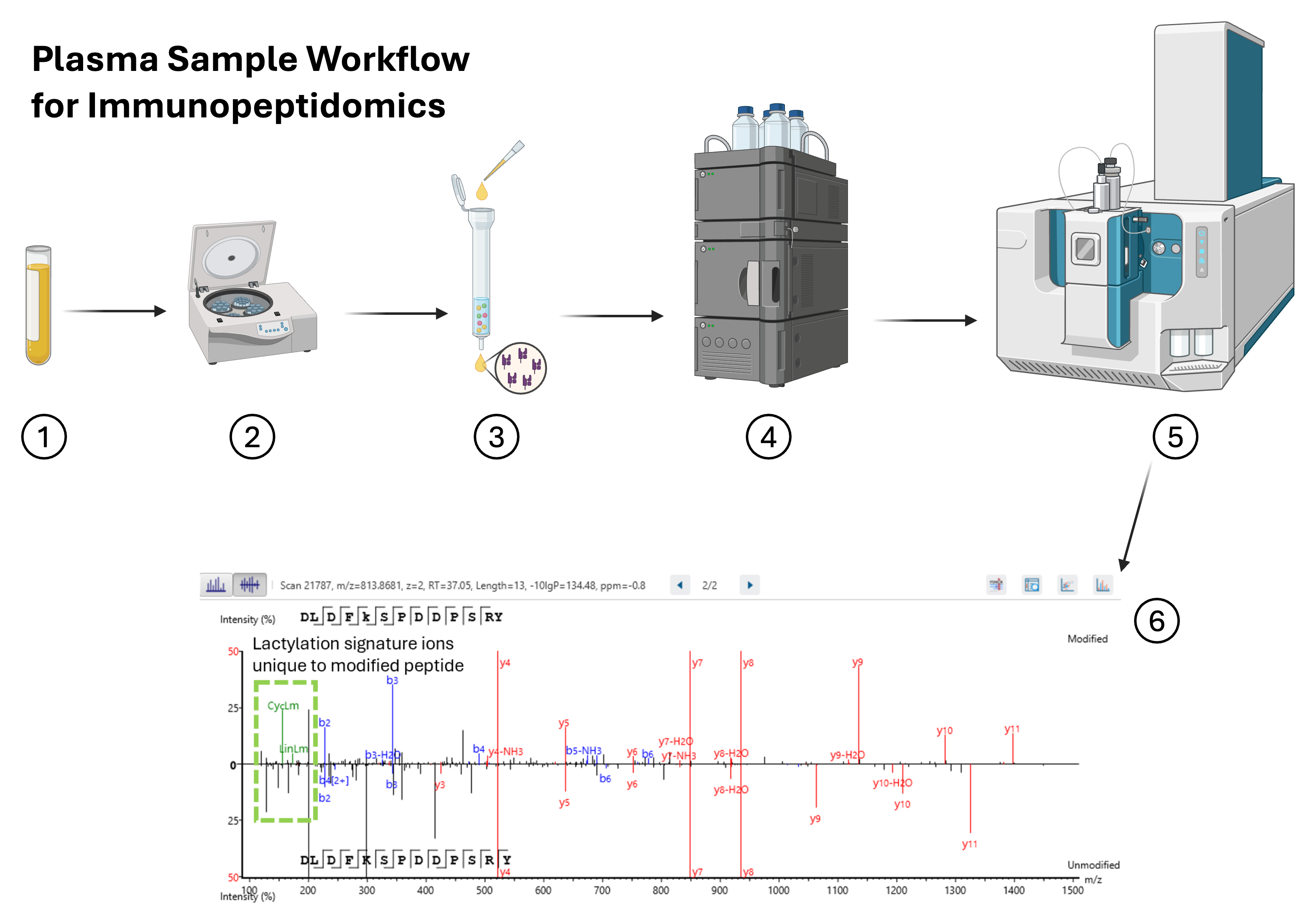
Schematic

  1. Obtain serum sample of plasma
  2. Spin out debris
  3. Run over IP column with anti-class I antibody
  4. Fractionate to purify peptides and exclude large proteins
  5. Use mass spec analysis software to obtain peptide sequences, source proteins, and genes
  6. Perform analysis

Analysis

Our lab is interested in looking at peak area and peak intensity to see if there are any COVID peptides or disease pathways present and detectable. Peak area is the total abundance throughout the entire sample and peak intensity is a relative abundance as a single ion hits the mass detector.

Workflow Schematic


Cool GIF [Link](https://warwick.ac.uk/fac/sci/lifesci/research/sigtraf/animations/):

Pathway and Gene Ontology Anylsis Packages Used

  • gprofiler2 Link
    • R package for g:Profiler tools g:GOst: Performs functional enrichment analysis
  • enrichR Link
    • Bioconductor package that gives you access to a suite of gene set enrichment analysis tools
  • clusterProfiler Link
    • Bioconductor package for any kind of “Omics” data interpretation: Annotation, Clustering, GO, GeneSetEnrichment, KEGG, MultipleComparison, Pathways, Reactome, Software, Visualization
  • enrichplot Link
    • Bioconductor package for visualization methods for interpreting functional enrichment results from ORA or GSEA analyses, for use with clusterProfiler and is based on ggplot

Get CSV Output from Mass Spec

# read in df
peptides <- read.csv("data/peptideDb.peptides.csv")

# glimpse df
glimpse(peptides)
Rows: 2,093
Columns: 28
$ Peptide               <chr> "A(+42.01)ANVTPADYAEWSK", "A(+42.01)ARPRDAL", "A…
$ X.10LgP               <dbl> 34.33, 24.95, 32.73, 34.15, 34.73, 27.77, 32.36,…
$ Mass                  <dbl> 1563.7205, 910.4984, 1010.6012, 1463.6544, 1962.…
$ Tag.Length            <int> 14, 8, 10, 14, 17, 15, 17, 16, 16, 13, 13, 13, 1…
$ CAA....               <dbl> 35.7, 37.5, 40.0, 28.6, 47.1, 46.7, 47.1, 62.5, …
$ Length                <int> 14, 8, 10, 14, 17, 15, 17, 16, 16, 13, 13, 13, 1…
$ Delta.RT              <chr> "-11.9480", "17.5813", "-77.7874", "8.5478", "-1…
$ MS2.Correlation       <dbl> 0.47, 0.10, 0.26, 0.41, 0.44, 0.68, 0.26, 0.04, …
$ ppm                   <dbl> -5.5, -2.0, 0.4, 1.8, 6.6, 0.3, -1.4, -8.9, 12.7…
$ m.z                   <dbl> 782.8632, 456.2556, 506.3080, 732.8373, 982.4172…
$ z                     <int> 2, 2, 2, 2, 2, 2, 2, 2, 3, 2, 2, 2, 2, 2, 2, 2, …
$ RT                    <dbl> 55.0110, 41.8248, 51.8708, 48.9945, 50.2847, 49.…
$ Area.Sample.1         <dbl> 306, NA, NA, 3180, 514, 518, 145, 5190, 1890, 69…
$ Intensity.Sample.1    <dbl> 1760, NA, NA, 14100, 4020, 4130, 760, 26600, 105…
$ Scan                  <int> 8569, 7615, 9622, 9244, 8495, 9448, 10047, 10860…
$ Source.File           <chr> "260717_1008_W632_070626_Fxn12.wiff", "260717_10…
$ X.Spec                <int> 1, 1, 3, 22, 7, 9, 4, 17, 7, 9, 103, 2, 4, 2, 3,…
$ X.Spec.Sample.1       <int> 1, 1, 3, 22, 7, 9, 4, 17, 7, 9, 103, 2, 4, 2, 3,…
$ X.Feature             <int> 1, 0, 0, 8, 2, 1, 1, 4, 5, 5, 31, 2, 1, 2, 3, 0,…
$ X.Feature.Sample.1    <int> 1, 0, 0, 8, 2, 1, 1, 4, 5, 5, 31, 2, 1, 2, 3, 0,…
$ Accession             <chr> "Biognosys|iRT-Kit_peptide_10:Q14517|FAT1_HUMAN"…
$ Gene                  <chr> "FAT1", "DNAAF5", "SCRIB", "", "", "", "", "SIGL…
$ Database              <chr> "TARGET", "TARGET", "TARGET", "TARGET", "TARGET"…
$ PTM                   <chr> "Acetylation (N-term)", "Acetylation (N-term)", …
$ AScore                <chr> "A1:Acetylation (N-term):1000.00", "A1:Acetylati…
$ Positional.Confidence <chr> "0 0 0 33 19 3 2 2 0 0 0 0 0 0", "0 0 0 0 0 7 7 …
$ tag...0.0..           <chr> "A(+42.01)ANVTPADYAEWSK", "A(+42.01)ARPRDAL", "A…
$ Found.By              <chr> "DeepNovo", "DB Search", "DB Search", "DeepNovo"…
Clean the Data

pep_clean <- peptides |>
  dplyr::select(Peptide, Length, Area.Sample.1, Intensity.Sample.1, Source.File, Accession, Gene, Found.By) |>
  mutate(Peptide = gsub("\\([^()]*\\)", "", Peptide)) |>
  mutate(accession_clean = sub("\\|.*", "", Accession)) |>
  filter(
    !str_detect(Accession, "Biognosys") &
    Found.By == "DB Search" &
    Length <= 14 &
    Length >= 8 &
    !str_detect(Peptide, "^[IL]+$")
  ) |>
  distinct(Peptide, .keep_all = TRUE) |>
  arrange(Length)

# Look at new cleaned df
head(pep_clean)
   Peptide Length Area.Sample.1 Intensity.Sample.1
1 AARPRDAL      8            NA                 NA
2 AAFEKQVL      8          1310              10600
3 APLLRWVL      8          9660              50800
4 APNLKSQL      8          2510              11900
5 DAVVKHVL      8            NA                 NA
6 DLGKKIAL      8          3690              20200
                         Source.File          Accession   Gene  Found.By
1 260717_1008_W632_070626_Fxn19.wiff Q86Y56|DAAF5_HUMAN DNAAF5 DB Search
2 260717_1008_W632_070626_Fxn18.wiff Q9P2E9|RRBP1_HUMAN  RRBP1 DB Search
3 260717_1008_W632_070626_Fxn26.wiff P09601|HMOX1_HUMAN  HMOX1 DB Search
4 260717_1008_W632_070626_Fxn17.wiff  Q9Y490|TLN1_HUMAN   TLN1 DB Search
5 260717_1008_W632_070626_Fxn16.wiff  P53621|COPA_HUMAN   COPA DB Search
6 260717_1008_W632_070626_Fxn18.wiff O94979|SC31A_HUMAN SEC31A DB Search
  accession_clean
1          Q86Y56
2          Q9P2E9
3          P09601
4          Q9Y490
5          P53621
6          O94979
# export csv to writes filepath
write.csv(pep_clean, "writes/clean_peptide_df.csv", row.names=FALSE)

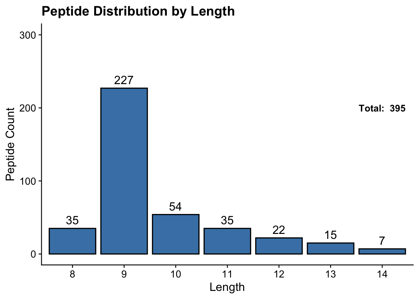
Visualize Peptide Distribution Based on Length

Code
# get total for annotation
total <- dim(pep_clean)[1]

# create x, y coordinates for annotation
annotations <- data.frame(
  x = 7,
  y = 200
)

# create label for annotation
label <- "Total: "

# Make length a factor variable for even distribution
pep_clean$Length <- factor(pep_clean$Length)

# plot
pep_dist_length <- pep_clean |> ggplot(aes(x = Length)) + 
  geom_bar(fill = "steelblue", color = "black") +
  geom_text(data = annotations, aes(x = x, y = y, label = paste(label, total)), 
            size = 4, fontface = "bold") +
  stat_count(geom = "text", aes(label = after_stat(count)), vjust = -0.5) +
  labs(title = "Peptide Distribution by Length",
       y = "Peptide Count") +
  ylim(0, 300) +
  theme_cowplot()

# visualize plot
pep_dist_length

Code
# save plot 
pep_dist_length |>
  ggsave(filename = "plots/dist_len.png", width = 8, height = 6, dpi = 300)

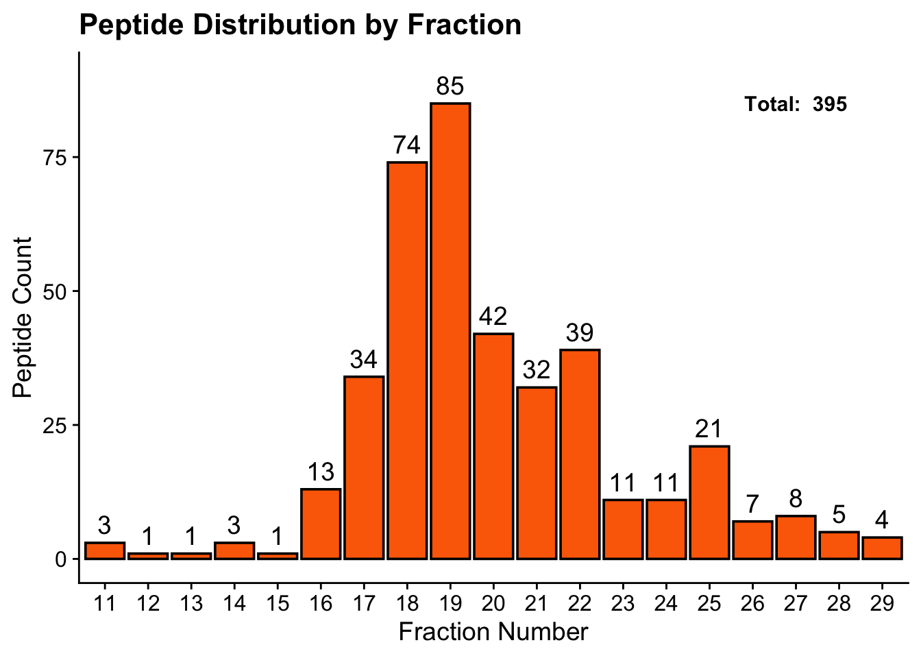
Visualize Peptide Distribution based on Fraction

Check for COVID-19 Peptides

# check for any accession value that does not contain human
non_human <- pep_clean |> filter(!str_detect(Accession, "HUMAN")) 
non_human
[1] Peptide            Length             Area.Sample.1      Intensity.Sample.1
[5] Source.File        Accession          Gene               Found.By          
[9] accession_clean   
<0 rows> (or 0-length row.names)
  • We weren’t able to identify any COVID-19 peptides from our extraction.

Identify 15 Most Abundant Peptides Overall Based on Peak Area

# select for top genes based on sample area
top_area_genes <- pep_clean |> 
  dplyr::select(Gene,accession_clean,Area.Sample.1) |>
  arrange(desc(Area.Sample.1))

top_area_genes$Gene[1:15]
 [1] "APOB"               "SLFN14"             "SAA4"              
 [4] "RPSA2:RPSA"         "C1QA"               "IGKV6D-21:IGKV6-21"
 [7] "IGHG1"              "HLA-C"              "HLA-C"             
[10] "SCP2"               "RNF213"             "TMED10"            
[13] "TTN"                "HP"                 "SYNCRIP:HNRNPR"    

Top 15 Most Abundant Peptides in COVID Sample

# select genes based on intensity
top_intensity_genes <- pep_clean |> 
  dplyr::select(Gene, accession_clean,Intensity.Sample.1) |>
  arrange(desc(Intensity.Sample.1))

top_intensity_genes$Gene[1:15]
 [1] "APOB"               "SLFN14"             "SAA4"              
 [4] "C1QA"               "HLA-C"              "RPSA2:RPSA"        
 [7] "HLA-C"              "IGKV6D-21:IGKV6-21" "IGHG1"             
[10] "SCP2"               "TMED10"             "RNF213"            
[13] "SYNCRIP:HNRNPR"     "LMO4"               "C1QC"              

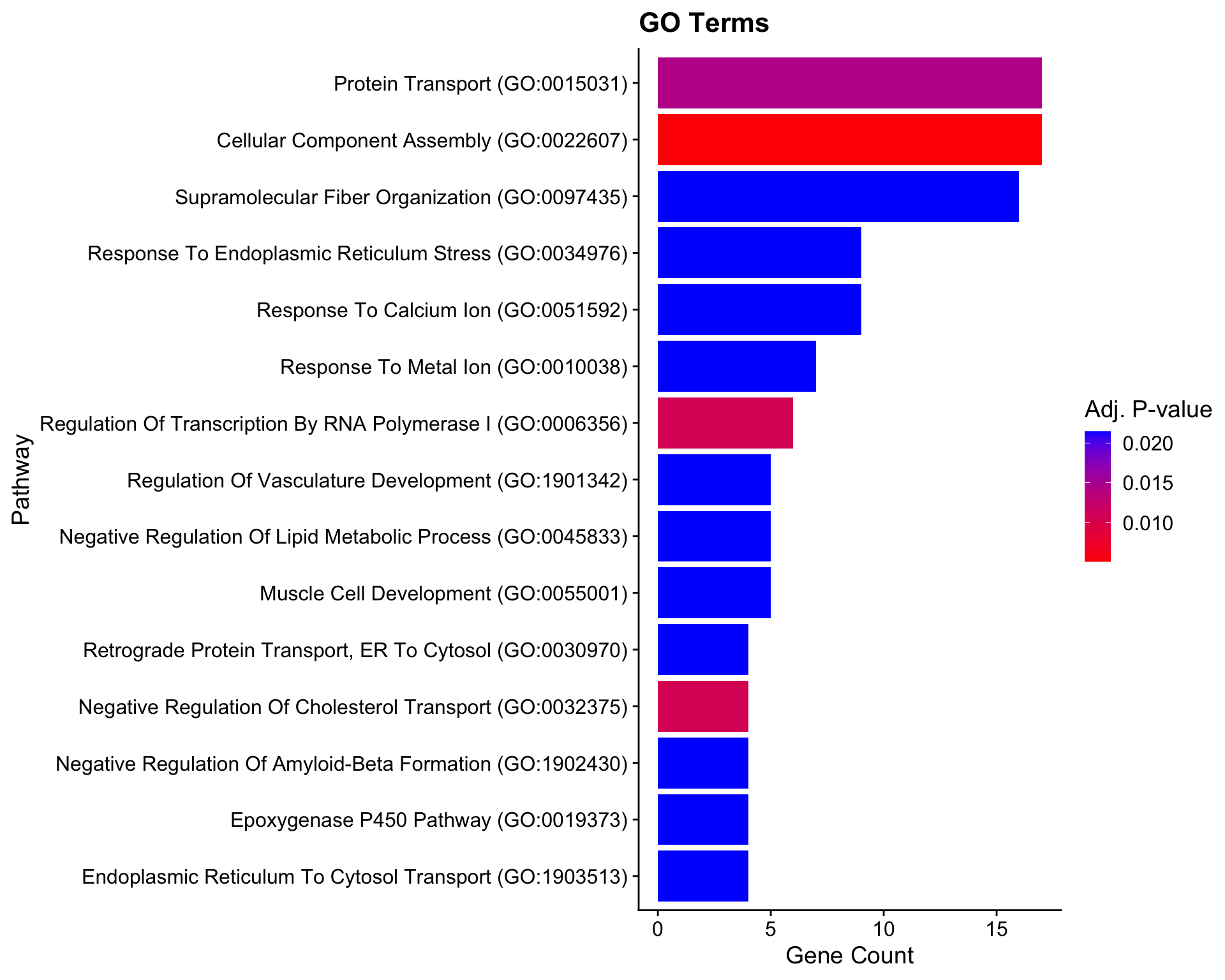
KEGG, Reactome, and GO Analysis

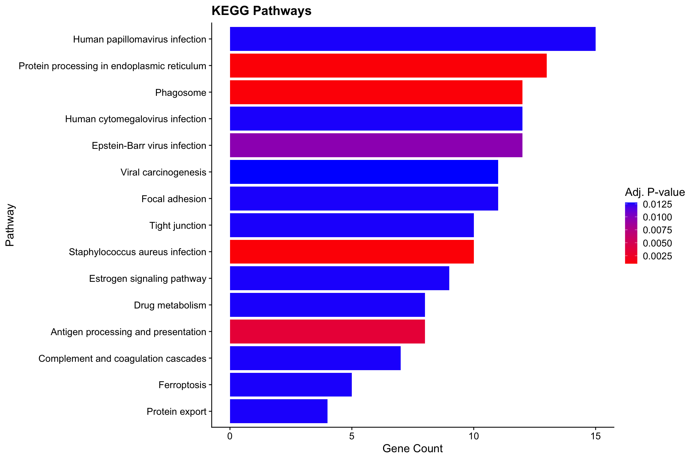
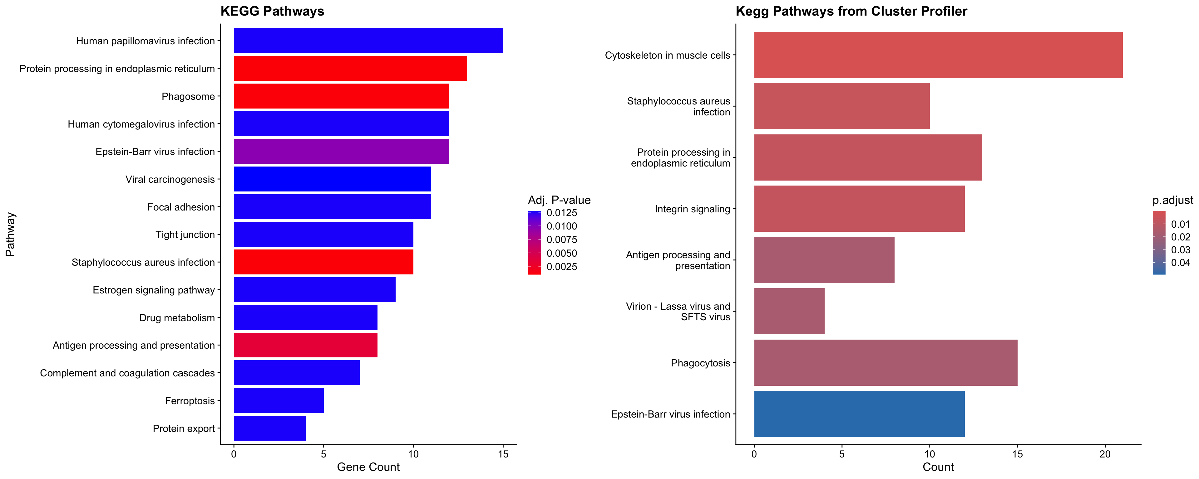
KEGG (Kyoto Encyclopedia of Genes and Genomes) Pathways Using gProfiler2

# view kegg pathways of enriched df
library(dplyr)
library(ggplot2)
library(tidyr)  

# select for top genes based on sample area
top_area_genes <- pep_clean |> 
  dplyr::select(Gene,accession_clean,Area.Sample.1) |>
  arrange(desc(Area.Sample.1))

genes <- top_area_genes$Gene

# get pathway from API for Gene column using gprofiler
gostres <- gost(query = genes,
                organism = "hsapiens",
                sources = c("GO:BP", "GO:MF", "GO:CC", "KEGG", "REAC"))

# use enrichR
dbs <- c("GO_Biological_Process_2023", "KEGG_2021_Human", "Reactome_2022")

# use gene term to identify terms
enriched <- enrichr(top_area_genes$Gene, dbs)
Uploading data to Enrichr... Done.
  Querying GO_Biological_Process_2023... Done.
  Querying KEGG_2021_Human... Done.
  Querying Reactome_2022... Done.
Parsing results... Done.
# Assuming your enrichR result for KEGG is called enrichr_kegg
plot_df <- enriched$KEGG_2021_Human |>
  # split "Overlap" (e.g. "5/120") into numeric gene count and pathway size
  separate(Overlap, into = c("Count", "Pathway.Size"), sep = "/", convert = TRUE) |>
  arrange(Adjusted.P.value) |>
  slice_head(n = 15)   # top 15 most significant pathways

kegg_abundant <-  ggplot(plot_df, aes(x = reorder(Term, Count), 
                     y = Count, 
                     fill = Adjusted.P.value)) +
  geom_col() +
  coord_flip() +
  scale_fill_gradient(low = "red", high = "blue") +  # low p-adj = red = more significant
  labs(x = "Pathway", y = "Gene Count", fill = "Adj. P-value",
       title = "KEGG Pathways") +
  theme_cowplot()

kegg_abundant

kegg_abundant |>
  ggsave(filename = "plots/kegg_abundant.png", width = 8, height = 6, dpi = 300)

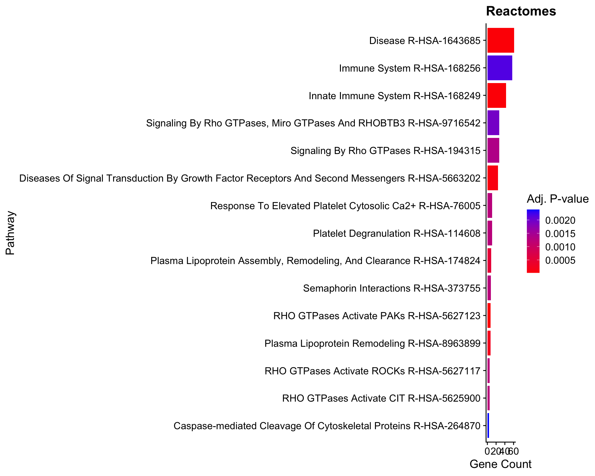
Reactomes

# Assuming your enrichR result for KEGG is called enrichr_kegg
plot_df <- enriched$Reactome_2022 |>
  # split "Overlap" (e.g. "5/120") into numeric gene count and pathway size
  separate(Overlap, into = c("Count", "Pathway.Size"), sep = "/", convert = TRUE) |>
  arrange(Adjusted.P.value) |>
  slice_head(n = 15)   # top 15 most significant pathways

reactome_abundant <- ggplot(plot_df, aes(x = reorder(Term, Count), 
                     y = Count, 
                     fill = Adjusted.P.value)) +
  geom_col() +
  coord_flip() +
  scale_fill_gradient(low = "red", high = "blue") +  # low p-adj = red = more significant
  labs(x = "Pathway", y = "Gene Count", fill = "Adj. P-value",
       title = "Reactomes") +
  theme_cowplot()

reactome_abundant

reactome_abundant |>
  ggsave(filename = "plots/reactome_abundant.png", width = 10, height = 8, dpi = 300)

Gene Ontology Terms

plot_df <- enriched$GO_Biological_Process_2023 |>
  # split "Overlap" into numeric gene count and pathway size
  separate(Overlap, into = c("Count", "Pathway.Size"), sep = "/", convert = TRUE) |>
  arrange(Adjusted.P.value) |>
  slice_head(n = 15)   # top 15 most significant pathways

GO_abundant <- ggplot(plot_df, aes(x = reorder(Term, Count), 
                     y = Count, 
                     fill = Adjusted.P.value)) +
  geom_col() +
  coord_flip() +
  scale_fill_gradient(low = "red", high = "blue") +  # low p-adj = red = more significant
  labs(x = "Pathway", y = "Gene Count", fill = "Adj. P-value",
       title = "GO Terms") +
  theme_cowplot()

# show plot

GO_abundant

# save plot
GO_abundant |>
  ggsave(filename = "plots/GO_abundant.png", width = 9, height = 8, dpi = 300)

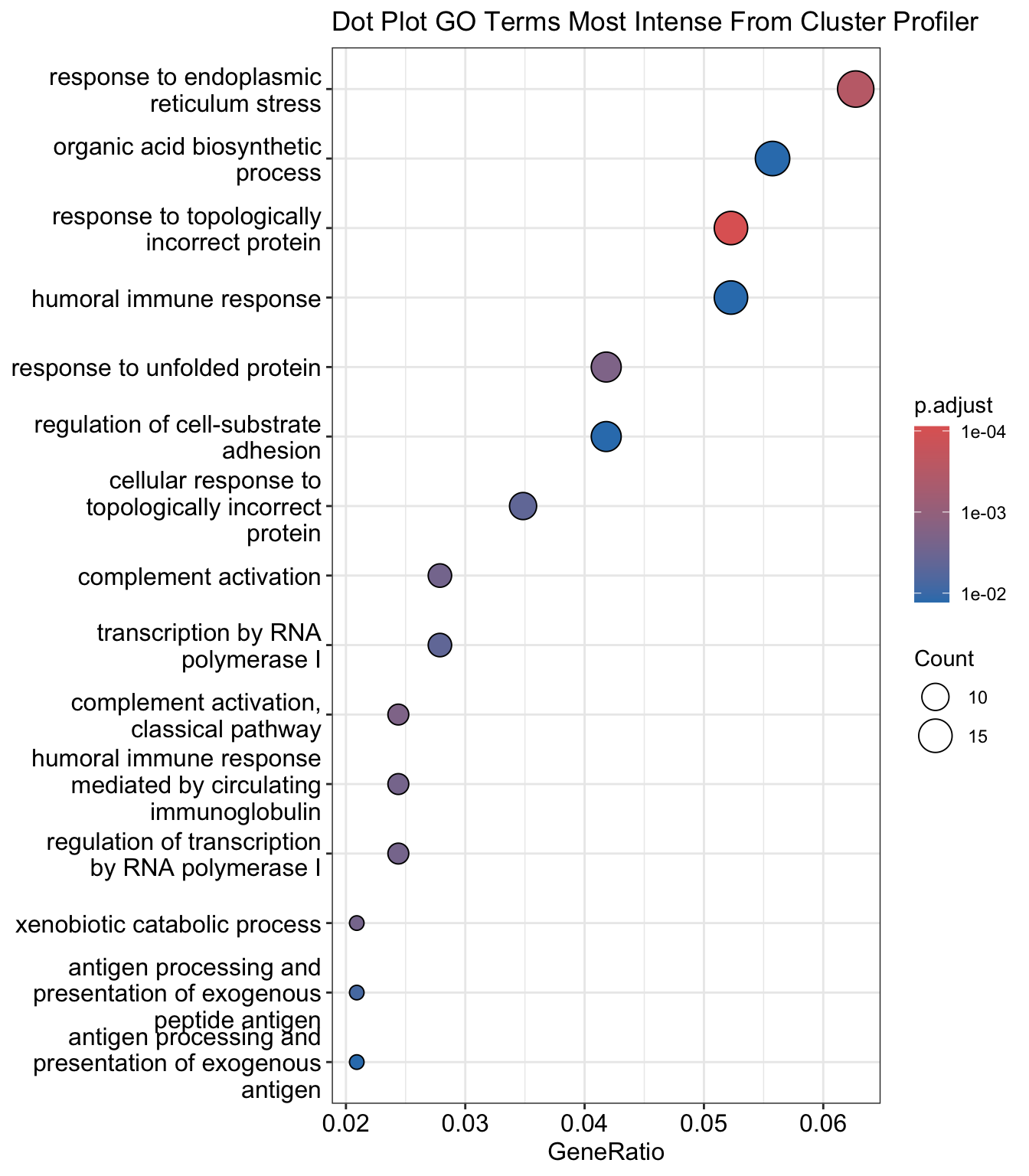
Use Cluster Profiler on for Most Intense Peptides

Code
# convert to entrez ids
id_map <- bitr(genes,
               fromType = "SYMBOL",
               toType   = "ENTREZID",
               OrgDb    = org.Hs.eg.db)
'select()' returned 1:1 mapping between keys and columns
Warning in bitr(genes, fromType = "SYMBOL", toType = "ENTREZID", OrgDb =
org.Hs.eg.db): 12.9% of input gene IDs are fail to map...
Code
# run enrichmnet analysis
go_enrich <- enrichGO(gene          = id_map$ENTREZID,
                       OrgDb         = org.Hs.eg.db,
                       keyType       = "ENTREZID",
                       ont           = "ALL",
                       pAdjustMethod = "BH",
                       pvalueCutoff  = 0.05,
                       qvalueCutoff  = 0.2,
                       readable      = TRUE)  

head(as.data.frame(go_enrich))
           ONTOLOGY         ID
GO:0035966       BP GO:0035966
GO:0034976       BP GO:0034976
GO:0006958       BP GO:0006958
GO:0006986       BP GO:0006986
GO:0002455       BP GO:0002455
GO:0006356       BP GO:0006356
                                                              Description
GO:0035966                    response to topologically incorrect protein
GO:0034976                       response to endoplasmic reticulum stress
GO:0006958                       complement activation, classical pathway
GO:0006986                                   response to unfolded protein
GO:0002455 humoral immune response mediated by circulating immunoglobulin
GO:0006356                regulation of transcription by RNA polymerase I
           GeneRatio   BgRatio RichFactor FoldEnrichment   zScore       pvalue
GO:0035966    15/287 161/18842 0.09316770       6.116606 8.108813 2.580537e-08
GO:0034976    18/287 269/18842 0.06691450       4.393042 6.970866 1.762684e-07
GO:0006958     7/287  39/18842 0.17948718      11.783615 8.383889 1.791623e-06
GO:0006986    12/287 145/18842 0.08275862       5.433233 6.664707 2.314093e-06
GO:0002455     7/287  44/18842 0.15909091      10.444568 7.800367 4.182451e-06
GO:0006356     7/287  45/18842 0.15555556      10.212466 7.694853 4.888886e-06
               p.adjust       qvalue
GO:0035966 8.791888e-05 6.787694e-06
GO:0034976 3.002733e-04 2.318231e-05
GO:0006958 1.971029e-03 1.521714e-04
GO:0006986 1.971029e-03 1.521714e-04
GO:0002455 2.518499e-03 1.944383e-04
GO:0006356 2.518499e-03 1.944383e-04
                                                                                                               geneID
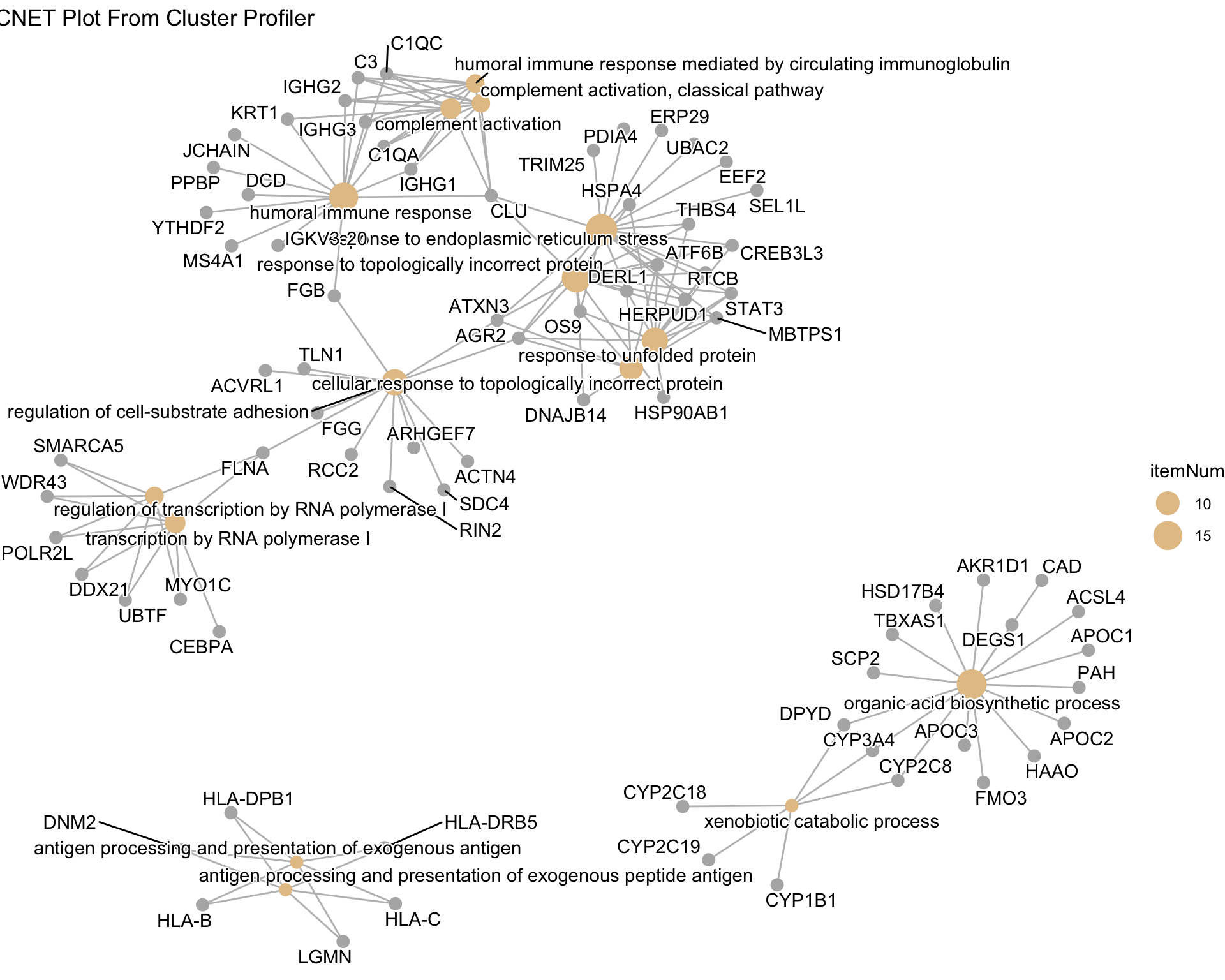
GO:0035966              RTCB/HERPUD1/DERL1/STAT3/AGR2/MBTPS1/HSP90AB1/CREB3L3/DNAJB14/OS9/HSPA4/CLU/THBS4/ATF6B/ATXN3
GO:0034976 RTCB/EEF2/UBAC2/HERPUD1/SEL1L/DERL1/ERP29/STAT3/TRIM25/AGR2/MBTPS1/PDIA4/CREB3L3/OS9/CLU/THBS4/ATF6B/ATXN3
GO:0006958                                                                         C1QC/C3/IGHG2/IGHG1/C1QA/CLU/IGHG3
GO:0006986                                RTCB/HERPUD1/DERL1/STAT3/AGR2/MBTPS1/HSP90AB1/CREB3L3/OS9/HSPA4/THBS4/ATF6B
GO:0002455                                                                         C1QC/C3/IGHG2/IGHG1/C1QA/CLU/IGHG3
GO:0006356                                                                 UBTF/FLNA/POLR2L/SMARCA5/WDR43/DDX21/MYO1C
           Count
GO:0035966    15
GO:0034976    18
GO:0006958     7
GO:0006986    12
GO:0002455     7
GO:0006356     7
Code
# run KEGG pathway analysis
kegg_enrich <- enrichKEGG(gene = id_map$ENTREZID, 
                          organism = "hsa", 
                          pvalueCutoff = 0.05)
Reading KEGG annotation online: "https://rest.kegg.jp/link/hsa/pathway"...
Reading KEGG annotation online: "https://rest.kegg.jp/list/pathway/hsa"...
Code
head(as.data.frame(kegg_enrich))
                                     category
hsa04820                   Cellular Processes
hsa05150                       Human Diseases
hsa04141       Genetic Information Processing
hsa04518 Environmental Information Processing
hsa04612                   Organismal Systems
hsa03273       Genetic Information Processing
                                 subcategory       ID
hsa04820                       Cell motility hsa04820
hsa05150       Infectious disease: bacterial hsa05150
hsa04141    Folding, sorting and degradation hsa04141
hsa04518 Signaling molecules and interaction hsa04518
hsa04612                       Immune system hsa04612
hsa03273   Information processing in viruses hsa03273
                                         Description GeneRatio  BgRatio
hsa04820                Cytoskeleton in muscle cells    21/200 233/9421
hsa05150             Staphylococcus aureus infection    10/200  99/9421
hsa04141 Protein processing in endoplasmic reticulum    13/200 175/9421
hsa04518                          Integrin signaling    12/200 154/9421
hsa04612         Antigen processing and presentation     8/200  82/9421
hsa03273         Virion - Lassa virus and SFTS virus     4/200  17/9421
         RichFactor FoldEnrichment   zScore       pvalue     p.adjust
hsa04820 0.09012876       4.245515 7.387586 2.023262e-08 5.746065e-06
hsa05150 0.10101010       4.758081 5.535803 4.476895e-05 6.357191e-03
hsa04141 0.07428571       3.499229 4.914728 8.673550e-05 7.322386e-03
hsa04518 0.07792208       3.670519 4.920826 1.031322e-04 7.322386e-03
hsa04612 0.09756098       4.595610 4.815936 3.330163e-04 1.698436e-02
hsa03273 0.23529412      11.083529 6.128189 3.776083e-04 1.698436e-02
               qvalue
hsa04820 3.218378e-06
hsa05150 3.560670e-03
hsa04141 4.101278e-03
hsa04518 4.101278e-03
hsa04612 9.512961e-03
hsa03273 9.512961e-03
                                                                                                              geneID
hsa04820 7431/23345/2006/79784/4627/6385/633/25777/5339/23002/6709/1287/6645/3675/4629/7094/7273/4633/7060/2023/6711
hsa05150                                                              2266/714/3115/718/3127/3857/3861/3858/712/6404
hsa04141                                        22872/5887/6238/9709/6400/79139/10961/8720/9601/3326/10956/1388/4287
hsa04518                                                     2266/2316/718/3914/1287/3675/1499/2244/81/7094/7060/896
hsa04612                                                                     3115/3107/3127/5641/3106/3326/3308/6890
hsa03273                                                                                        79784/4627/4629/8828
         Count
hsa04820    21
hsa05150    10
hsa04141    13
hsa04518    12
hsa04612     8
hsa03273     4
Code
# run reactome analysis
reactome_enrich <- enrichPathway(gene         = id_map$ENTREZID,
                                  organism     = "human",
                                  pvalueCutoff = 0.05,
                                  readable     = TRUE)

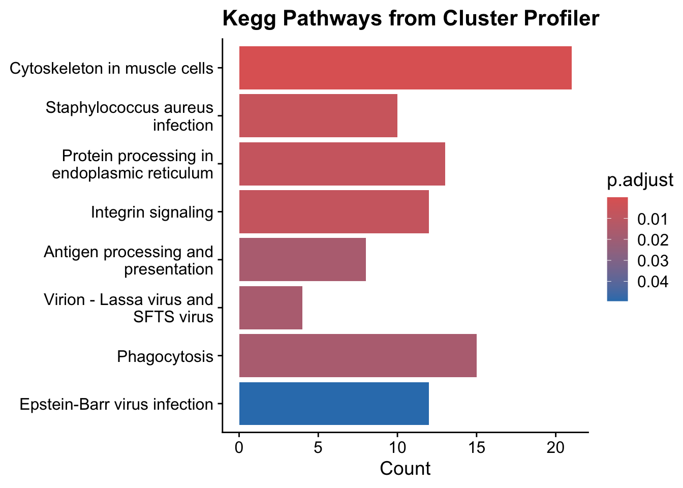
Kegg Pathways From Cluster Profiler for Most Intense Peptides

# use enrichplot barplot to show Kegg pathways with most significant 
kegg_cluster <- barplot(kegg_enrich, showCategory = 15) + 
  ggtitle("Kegg Pathways from Cluster Profiler") +
  theme_cowplot()
kegg_cluster

Side by Side gprofiler2 and clusterProfiler KEGG Pathways
plot_grid(kegg_abundant, kegg_cluster)

GO Terms From Cluster Profiler for Most Intense Peptides

# change fig size

# create plot variable
dot_cluster <- dotplot(go_enrich, showCategory = 15, title="Dot Plot GO Terms Most Intense From Cluster Profiler", font.size = 12) 

# display dot plot of GO terms
dot_cluster 

# save plot
dot_cluster |>  ggsave(filename = "plots/dot_cluster.png", width = 7, height = 9, dpi = 300)

CNet Plot from Cluster Profiler for Most Intense Peptides

# create plot variable
cnet_cluster <- cnetplot(go_enrich, showCategory = 15) + 
  ggtitle("CNET Plot From Cluster Profiler")

# display plot
cnet_cluster

# save plot
cnet_cluster |> ggsave(filename = "plots/cnet_cluster.png", width = 10, height = 8, dpi = 300)

Conclusions

  • Originally ~2000 peptides were identified, but upon filtering them down there were really only 395 confidently identified peptides that matched documented human database genes/proteins
  • No well-documented COVID-19 peptides were identified 😔 (there are only 17 well documented proteins for SARS CoV-2 which are all from the Wuhan strain and don’t take into account variants or mutations to proteins)
  • Pathway analysis revealed other viral response related proteins to be over-represented in sHLA Class I
    • maybe the COVID response related proteins are not as well characterized as others
    • sHLA does not slough off into the plasma as well for COVID infected cells or COVID prevents this
    • COVID may interfere with class I processing or presentation

Future Direction

  • Currently have another sHLA Class I sample from a COVID infected patient being run on the mass spec set to finish 07/29/2026 @10PM
  • Could potentially be a diagnostic of some sort